Formulas and Functions: How to Make Calculations in Excel

Spreadsheets are an amazing tool for calculations. The possibilities are endless, ranging from basics, such as summing expenses, to sophisticated statistics. To get you started on this, you will need to understand how to build a formula in Excel and how it differentiates between a formula and a function.

Formula vs Function

The term formula is used for any type of formula you make up manually. Formulas should still contain cell references as this will allow Excel to recalculate the result whenever you make adjustments in a cell. The counterpart of formulas are functions. Those are are build-in features in Excel (and other spreadsheet applications). Compared to formulas, functions allow for easier and more advanced spreadsheet manipulation. An example of a function is =SUM(), which will automatically sum up the numbers or cell references within the brackets. As long as you use cell references, Excel will automatically update the results of both formulas and functions.

How to enter a Formula or Function

There are two methods to enter formulas and functions. With one you will primarily (or exclusively) work with is up to you. Personally, I use a mix of both methods, but more on that later, which I will go into a bit more later.

Let’s say you have a file with sales data. In column C you have the quantity that was sold for a specific item on that day. In column D you have the unit price (price per single item). Now you would like to calculate how much the total price for each sale was. This calculation takes place in column E. Let’s look at the two methods to enter a formula:

Method 1

1. Double click the cell you wish to edit. You will now see the blinking cursor in that cell, signalling Excel is ready for you to type.
2. Every formula and function starts out with the equal sign, followed by the operation you wish to do.
3. Adding a cell reference is as easy as clicking on the relevant cell. Don’t forget the mathematical operation symbols in-between cell references so Excel knows what it’s supposed to do.
4. Click enter once you’re done. Excel will now show you the result.

Method 2

The other way to enter a formula is by using the formula bar which is located between the menu ribbon and the spreadsheets’ content. This replaces step 1 in the first method. Steps 2 to 4 are still the same.

Formula Builder

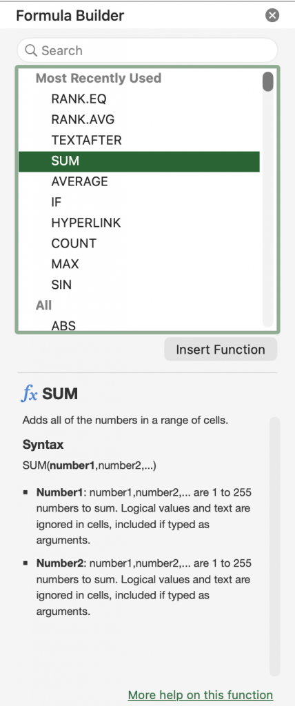
Another useful tool Excel offers is the Formula Builder. This feature offers a function search bar, a step-by-step guide on the selected function and a link to the Microsoft website where more help on the function is offered. The Formula Builder is really more of a function builder rather than a ‘manual’ formula builder. As you might have guessed now, sometimes the words can be used interchangeably.

How to access the Formula Builder

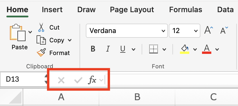
Make sure you have selected the cell in which you wish to enter a function. Then click on the button labelled fx located to the left of the formula bar.

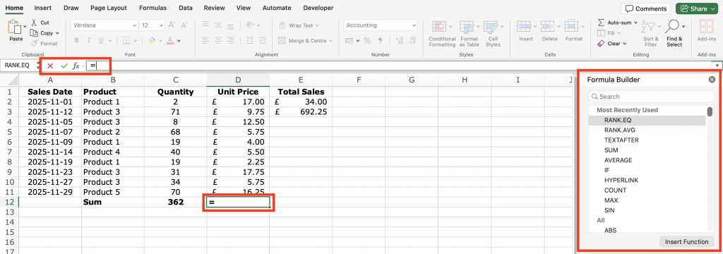
After clicking fx Excel automatically started the formula by entering = into the formula bar. To the right of your screen you will see a menu that opened up now. That is the Formula Builder. By default it shows you your Most Recently Used function and an alphabetical list with All available functions underneath it.

Additional Note: To the left of the fx button you can see the x and confirm-tick are now coloured in while before they have been greyed out. Clicking on either button will either cancel or confirm the changes you have made in the formula bar. Alternatively you can press enter (to confirm) or escape (to cancel the changes).

You can either select a function from the suggested options or use the search bar to find what you are looking for (see left-hand screenshot below). Clicking on a function name once will highlight its name. Double clicking will select the function and bring you to its Formula Builder (see right-hand screenshot below).

In the example below I selected the SUM function. As I had cell D12 selected which is beneath the Unit Price entries for the products shown in my example, Excel auto-suggests that I sum up the Unit Prices in cells D2:D11 (see below the label Number1). If that is what I wish to do, I can confirm by pressing on Done.

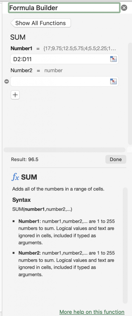
Another helpful feature to point out is the numeric preview in the Formula Builder. Next to Number1 you will see the number values 17, 9.75, 12.5 and so on. Comparing them with the numbers in my screenshot above you will notice that these numbers represent the values in the selected cells, in the order of their appearance. In the Formula Builder to the left of the Done button Excel also adds the Result which is 96.5 in this case. Having these previous lets you double check that the formula you have created does what you want it to do.